7. Adams-Bashforth Multistep Methods

Note. For now, the examples are done with the Julia language; a Python translation is coming soon.

References:

• Section 6.7 Multistep Methods of Sauer

• Section 5.6 Multistep Methods of Burden&Faires

7.1. Introduction

Recall from An Introduction to Multistep Methods: Leap-frog:

Definition: A multistep method for numerical solution of an ODE IVP \(du/dt = f(t, u)\), \(u(t_0) = u_0\) is one of the form

\[U_{i} = \phi(U_{i-1}, \dots U_{i-s}, h), \quad s > 1\]

so that the new approximate value of \(u(t)\) depends on approximate values at multiple previous times. (The shift if indexing to describe “present” in terms of “past” wil be convenient here.)

This is called an \(s\)-step method: the Runge-Kutta family of methods are all one-step.

We will be more specifically interted in what are called linear multistep methods, where the function at right is a linear combination of value of \(u(t)\) and \(f(t, u(t))\).

So for now we look at

\[U_{i} = a_0 U_{i-s} + \dots + a_{s-1} U_{i-1} + h (b_0 f(t_{i-s}, U_{i-s}) + \dots + b_{s-1} f(t_{i-1}, U_{i-1})) \]

The Adams-Bashforth methods are a case of this with the only \(a_i\) term being \(a_{s-1} = 1\):

\[U_{i} = U_{i-1} + h (b_0 f(t_{i-s}, U_{i-s}) + \dots + b_{s-1} f(t_{i-1}, U_{i-1})) \]

The \(s\)-step versions of this is accurate to order \(s\), so one can get arbitrarily high order of accuracy by using enough steps.

Aside: the case \(s=1\) is Euler’s method, now written as

\[U_{i} = U_{i-1} + h f(t_{i-1}, U_{i-1})\]

These are probably the most commonly used explicit, one-stage multi-step methods; we will see more about the alternatives of implicit and multi-stage options in future sections. (Note that all Runge-Kutta methods (except Euler’s) are multi-stage: the explicit trapezoid and midpoint methods are 2-stage; the classical Runge-Kutta method is 4-stage.)

The most basic Adams-Bashforth multi-step method is the 2-step method, which can be thought of this way:

1. Start with the two most recent values, \(U_{i-1} \approx u(t_{i) - h}\) and \(U_{i-2} \approx u(t_i - 2h)\)

2. Use the derivative approximations \(F_{i-1} := f(t_{i-1}, U_{i-1}) \approx u'(t_{i-1})\) and \(F_{i-2} := f(t_{i-2}, U_{i-2}) \approx u'(t_{i-2})\) and linear extrapolation to “predict” the value of \(u'(t_i - h/2)\); one gets: \(u'(t_i - h/2) \approx \frac{3}{2} u'(t_i - h) - \frac{1}{2}u'(t_i - 2h) \approx \frac{3}{2} F_{i-1} - \frac{1}{2}F_{i-2}\)

3. Use this in the centered difference approximation

\[\frac{u(t_{i}) - u(t_{i-1})}{h} \approx u'(t_i - h/2)\]

to get

\[\frac{U_{i} - U_{i-1}}{h} \approx \frac{3}{2} F_{i-1} - \frac{1}{2} F_{i-2}\]

That is,

\[ U_{i} = U_{i-1} + \frac{h}{2} \left( 3 F_{i-1} - F_{i-2} \right), = U_{i-1} + \frac{h}{2} \left( 3 f(t_{i-1}, U_{i-1}) - f(t_{i-2}, U_{i-2}) \right) \]

Equivalently, one can

1. Find the collocating polynomial \(p(t)\) through \((t_{i-1}, F_{i-1})\) and \((t_{i-2}, F_{i-2})\) [so just a line in this case]

2. Use this on the interval \((t_{i-1}, t_{i})\) (extrapolation) as an approximation of \(u'(t) = f(t, u(t))\) in that interval.

3. Use \(\displaystyle u(t_{i}) = u(t_{i-1}) + \int_{t_{i-1}}^{t_{i}} u'(\tau) d \tau \approx u(t_{i-1}) + \int_{t_{i-1}}^{t_{i}} p(\tau) d \tau\), where the latter integral is easy to evaluate exactly.

One does not actually do this in each case; it is enough to verify that the integral gives \((3/2 F_{i-1} - 1/2 F_{i-2}) h\).

---

Exercise A

Verify the above result via polynomial collocation and integration.

---

To code this algorithm, it is convenient to shift the indices, to get a formula for \(U_i\). Also, note that what is \(F_i = f(t_i, U_i)\) at one step is reused as \(F_{i-1} = f(t_{i-1}, U_{i-1})\) at the next, so to avoid redundant evaluations of \(f(t, u)\), these quantities should also be saved, at least till the next step:

\[U_{i} = U_{i-1} + \frac{h}{2} \left( 3 F_{i-1} - F_{i-2} \right)\]

using PyPlot

include("NumericalMethods.jl")
import .NumericalMethods as NM

function adamsbashforth2(f, a, b, U_0, U_1, n)
    n_unknowns = length(U_0)
    t = range(a, b, n+1)
    u = zeros(n+1, n_unknowns)
    u[1,:] = U_0
    u[2,:] = U_1
    F_i_2 = f(a, U_0)  # F_0 to start when computing U_2
    h = (b-a)/n
    for i in 2:n  # i is the mathematical index, so "+1" for Julia array indices
        F_i_1 = f(t[i], u[i,:])
        u[i+1,:] = u[i,:] + (3*F_i_1 - F_i_2) * (h/2)
        F_i_2 = F_i_1
    end
    return (t, u)
end;

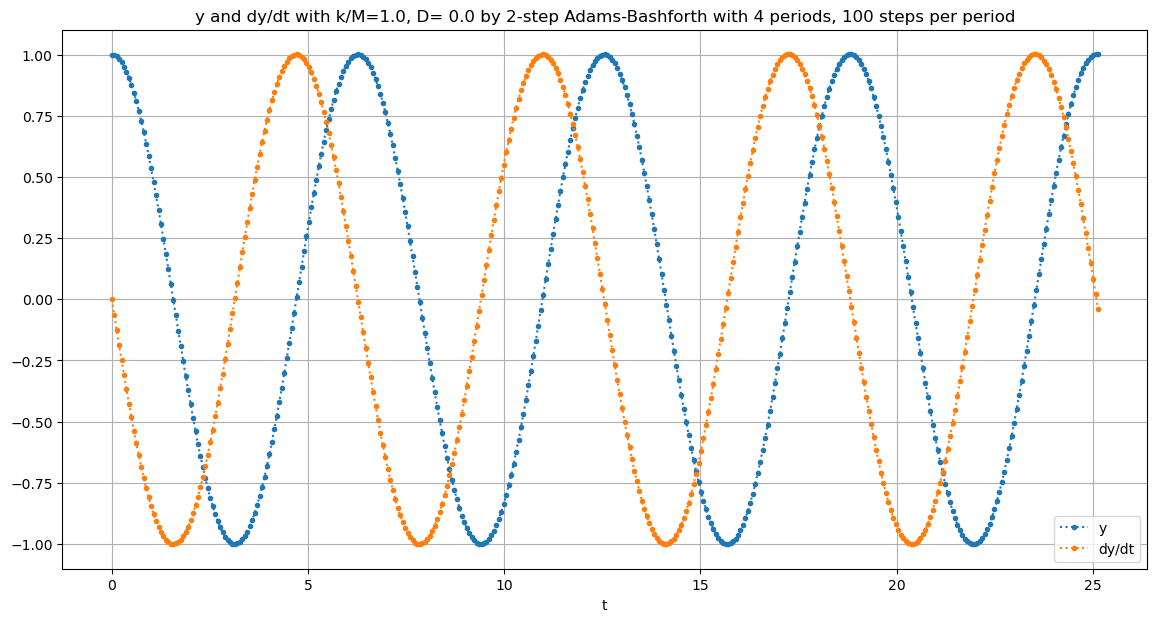
Demonstrations with the mass-spring system

f_mass_spring(t, u) = [ u[2]; -(k/M)*u[1] - (D/M)*u[2] ];

M = 1.0
k = 1.0
D = 0.0
U_0 = [1.0, 0.0]
a = 0.0
periods = 4
b = 2pi * periods

# Using a step size that gives roughly equal cost per unit time as for the explicit trapezoid and midpoint,
# Runge-Kutta methods and the leapfrog FAdams-Bmethod in previous sections
stepsperperiod = 100  
n = Int(stepsperperiod * periods)

# We need U_1, and get it with the Runge-Kutta method;
# this is overkill for accuracy, but since only one step is needed, the time cost is negligible.
h = (b-a)/n
(t_1step, U_1step) = NM.rungekutta_system(f_mass_spring, a, a+h, U_0, 1)
U_1 = U_1step[end,:]
(t, U) = adamsbashforth2(f_mass_spring, a, b, U_0, U_1, n)

y = U[:,1]
Dy = U[:,2]

figure(figsize=[14,7])
title("y and dy/dt with k/M=$(k/M), D= $D by 2-step Adams-Bashforth with $periods periods, $stepsperperiod steps per period")
plot(t, y, ".:", label="y")
plot(t, Dy, ".:", label="dy/dt")
legend()
xlabel("t")
grid(true)

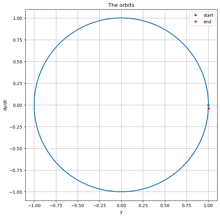
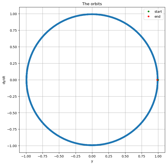
figure(figsize=[8,8])  # Make axes equal length; orbits should be circular or "circular spirals"
title("The orbits")
plot(y, Dy)
xlabel("y")
ylabel("dy/dt")
plot(y[1], Dy[1], "g*", label="start")
plot(y[end], Dy[end], "r*", label="end")
legend()
grid(true)

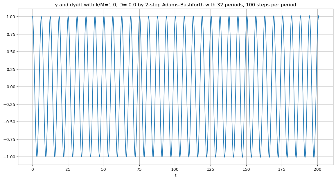
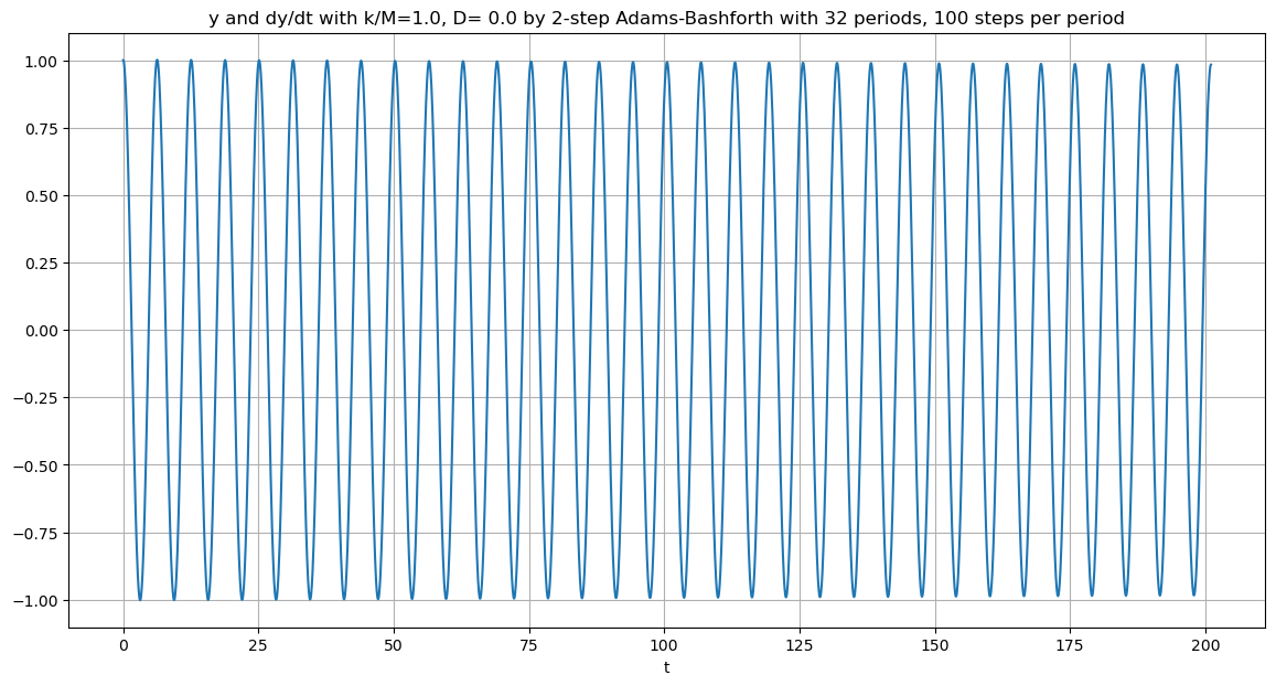
D = 0.0

periods = 32
b = 2pi * periods

# Note: In the notes on systems, the second order methods were tested with 50 steps per period
#stepsperperiod = 50  # As for the second order accurate explicit trapezoid and midpoint methods
stepsperperiod = 100  # Equal cost per unit time as for the explicit trapezoid and midpoint and Runge-Kutta methods
n = Int(stepsperperiod * periods)

# We need U_1, and get it with the Runge-Kutta method;
# this is overkill for accuracy, but since only one step is needed, the time cost is negligible.
h = (b-a)/n
(t_1step, U_1step) = NM.rungekutta_system(f_mass_spring, a, a+h, U_0, 1)
U_1 = U_1step[end,:]
(t, U) = adamsbashforth2(f_mass_spring, a, b, U_0, U_1, n)

y = U[:,1]
Dy = U[:,2]

figure(figsize=[14,7])
title("y and dy/dt with k/M=$(k/M), D= $D by 2-step Adams-Bashforth with $periods periods, $stepsperperiod steps per period")
plot(t, y, label="y")
xlabel("t")
grid(true)

figure(figsize=[8,8])  # Make axes equal length; orbits should be circular or "circular spirals"
title("The orbits")
plot(y, Dy)
xlabel("y")
ylabel("dy/dt")
plot(y[1], Dy[1], "g*", label="start")
plot(y[end], Dy[end], "r*", label="end")
legend()
grid(true)

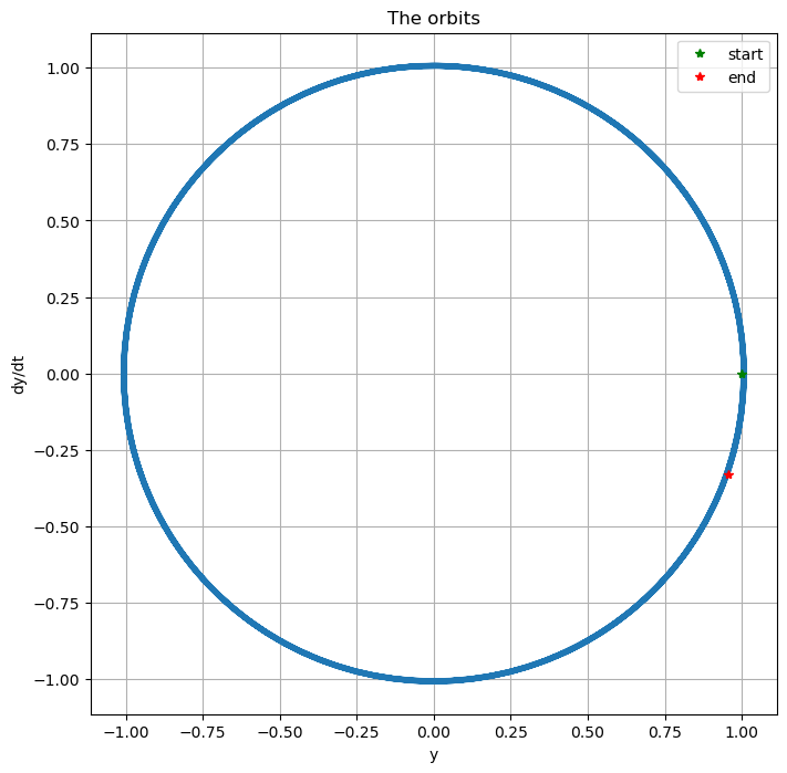
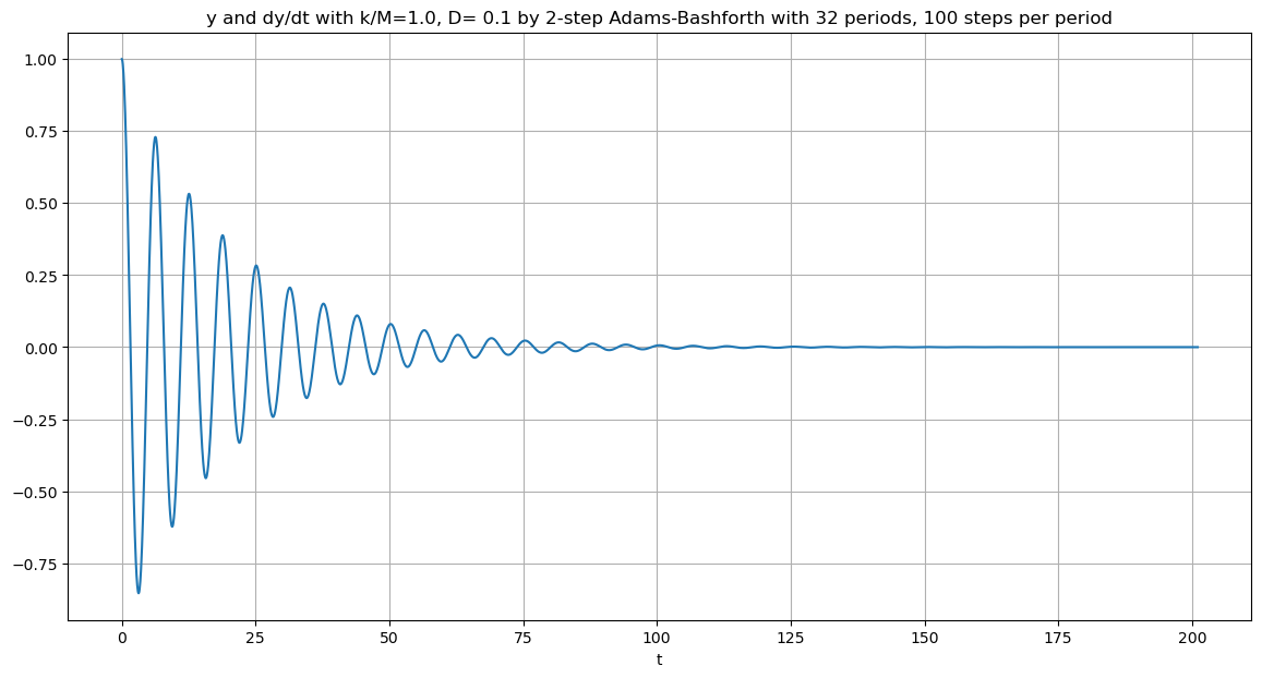
This time with damping, nothings goes wrong!

This is an example in stability; in future sections it will be seen that the the Adams-Bashforth methods are all stable for these equations for small enough step size \(h\), and so converge to the correct solution as \(h \to 0\).

D = 0.1

periods = 32
b = 2pi * periods

# We need U_1, and get it with the Runge-Kutta method;
# this is overkill for accuracy, but since only one step is needed, the time cost is negligible.
h = (b-a)/n
(t_1step, U_1step) = NM.rungekutta_system(f_mass_spring, a, a+h, U_0, 1)
U_1 = U_1step[end,:]
(t, U) = adamsbashforth2(f_mass_spring, a, b, U_0, U_1, n)

y = U[:,1]
Dy = U[:,2]

figure(figsize=[14,7])
title("y and dy/dt with k/M=$(k/M), D= $D by 2-step Adams-Bashforth with $periods periods, $stepsperperiod steps per period")
plot(t, y, label="y")
xlabel("t")
grid(true)

7.2. Higher order Adams-Bashforth methods

The strategy descibed about of polynomal approximation, extrapolaot oand integration can be generalized to get the \(s\) step admas-Bashforth method, of order \(s\); to get approximation \(U_i\) of \(u(t_i)\) from data at the \(s\) most recent previous times \(t_{i-1}\) to \(t_{i-s}\):

1. Find the collocating polynomial \(p(t)\) of degree \(s-1\) through \((t_{i-1}, F_{i-1}) \dots (t_{i-s}, F_{i-s})\)

2. Use this on the interval \((t_{i-1}, t_{i})\) (extrapolation) as an approximation of \(u'(t) = f(t, u(t))\) in that interval.

3. Use \(u(t_{i}) = u(t_{i-1}) + \int_{t_{i-1}}^{t_{i}} u'(\tau) d \tau \approx u(t_{i-1}) + \int_{t_{i-1}}^{t_{i}} p(\tau) d\tau\), where the latter integral can be evaluated exactly.

However, one does not actually evaluate this integral; it is enough to verify that the resultig form will be

\[U_{i} = U_{i-1} + h (b_0 F_{i-s} + b_1 F_{i-s+1} + \cdots b_{s-1} F_{i-1})\]

with the coefficients being the same for any \(f(t, u)\) and any \(h\).

Then they can be derived by the method of undetermined coefficients as seen in Approximating Derivatives by the Method of Undetermined Coefficients: insert Taylor polynomial approximations of \(u(t_{i-k}) = u(t_i) - k h)\) and \(f(t_{i-k}, u(t_{i-k})) = u'(t_{i-k}) = u'(t_i - k h)\) and solve for the \(s\) coefficients \(b_0 \dots b_{s-1}\) that give the highest power for the residual error. The terms in the first \(s\) powers of \(h\) (from 1 to \(h^{s-1}\)) can be cancelled leaving an error \(O(h^s)\).

\[U_{i} = U_{i-1} + h (b_0 f(t_{i-s}, U_{i-s}) + \dots + b_{s-1} f(t_{i-1}, U_{i-1})) \]

The first few are:

• \(s=1\): \(b_0 = 1, \quad U_{i} = U_{i-1} + h F_{i-1} = U_{i-1} + h f(t_{i-1}, U_{i-1})\) (Euler’s method)

• \(s=2\): \(b_0 = -1/2, b_1 = 3/2, \quad U_{i} = U_{i-1} + \frac{h}{2} \left( 3 F_{i-1} - F_{i-2} \right)\) (as above)

• \(s=3\): \(b_0 = 5/12, b_1 = -16/12, b_2 = 23/12, \quad U_{i} = U_{i-1} + \frac{h}{12} \left( 23 F_{i-1} - 16F_{i-2} + 5 F_{i-3} \right)\)

function adamsbashforth3(f, a, b, U_0, U_1, u_2, n)
    n_unknowns = length(U_0)
    t = range(a, b, n+1)
    u = zeros(n+1, n_unknowns)
    u[1,:] = U_0
    u[2,:] = U_1
    u[3,:] = U_2
    F_i_3 = f(a, U_0)  # F_0 to start when computing U_3
    F_i_2 = f(a, U_1)  # F_1 to start when computing U_3
    h = (b-a)/n
    for i in 2:n  # i is the mathematical index, so "+1" for Julia array indices
        F_i_1 = f(t[i], u[i,:])
        u[i+1,:] = u[i,:] + (23F_i_1 - 16F_i_2+5F_i_3) * (h/12)
        (F_i_2, F_i_3) = (F_i_1, F_i_2)
    end
    return (t, u)
end;

D = 0.0

periods = 32
b = 2pi * periods

# Note: In the notes on systems, the second order methods were tested with 50 steps per period
#stepsperperiod = 50  # As for the second order accurate explicit trapezoid and midpoint methods
stepsperperiod = 100  # Equal cost per unit time as for the explicit trapezoid and midpoint and Runge-Kutta methods
n = Int(stepsperperiod * periods)

# We need U_1 and U_2, and get them with the Runge-Kutta method;
# this is overkill for accuracy, but since only two steps are needed, the time cost is negligible.
h = (b-a)/n
(t_2step, U_2step) = NM.rungekutta_system(f_mass_spring, a, a+2h, U_0, 2)
U_1 = U_2step[2,:]
U_2 = U_2step[3,:]
(t, U) = adamsbashforth3(f_mass_spring, a, b, U_0, U_1,U_2, n)

y = U[:,1]
Dy = U[:,2]

figure(figsize=[14,7])
title("y and dy/dt with k/M=$(k/M), D= $D by 2-step Adams-Bashforth with $periods periods, $stepsperperiod steps per period")
plot(t, y, label="y")
xlabel("t")
grid(true)

figure(figsize=[8,8])  # Make axes equal length; orbits should be circular or "circular spirals"
title("The orbits")
plot(y, Dy)
xlabel("y")
ylabel("dy/dt")
plot(y[1], Dy[1], "g*", label="start")
plot(y[end], Dy[end], "r*", label="end")
legend()
grid(true)

---

Exercise B

Verify the above result for \(s=3\) by the method of undetermined coefficients.

---

This work is licensed under Creative Commons Attribution-ShareAlike 4.0 International