4. Systems of ODEs and Higher Order ODEs

References:

• Section 6.3 Systems of Ordinary Differential Equations in Sauer, just to Sub-section 6.3.1 Higher order equations.

• Section 5.9 Higher Order Equations and Systems of Differential Equations in Burden&Faires

The short version of this section is that the numerical methods and algorithms developed so for for the initial value problem

\[\begin{split} \begin{split} \frac{d u}{d t} &= f(t, u(t)), \quad a \leq t \leq b \\ u(a) &= u_0 \end{split} \end{split}\]

all also work for system of first order ODEs by simply letting \(u\) and \(f\) be vector-valued, and for that, the Python code requires only one small change.

Also, higher order ODE’s (and systems of them) can be converted into systems of first order ODEs.

The second point is seen in a typical first course in differential equations, so I will just illustrate the procedure for a single famous example.

import numpy as np
# Shortcuts for some favorite commands:
from matplotlib.pyplot import figure, plot, grid, title, xlabel, ylabel, legend, show
from numpy import linspace

4.1. Motion of a Damped Mass-Spring System in One Dimension

A simple mathematical model of a damped mass-spring system is

\[\begin{split} \begin{split} M \frac{d^2 y}{d t^2} &= -k u - D \frac{d y}{d t} \\ & \text{with initial conditions} \\ y(a) &= y_0 \\ \left. \frac{dy}{dt} \right|_{t=a} &= v_0 \end{split} \end{split}\]

where \(k\) is the spring constant and \(D\) is the coefficient of friction, or drag.

To convert to a first order system, introduction the two functions

\[\begin{split} \begin{split} u_0(t) &= y(t) \\ u_1(t) &= \frac{d y}{d t} \end{split} \end{split}\]

(Aside: this is one of many places where the Pythonic system of counting from \(0\) fits the mathematics better!)

Then with \(d^2 y/dt^2 = d u_1/dt\) the above equation becomes

\[ \frac{d u_1}{d t} = -\frac{k}{M} u_0 - \frac{D}{M} u_1 \]

Combined with the definition of \(u_1\) give the system

\[\begin{split} \begin{split} \frac{d u_0}{d t} &= u_1 \\ \frac{d u_1}{d t} &= -\frac{k}{M} u_0 - \frac{D}{M} u_1 \\ &\text{with initial conditions} \\ u_0(a) &= y_0 \\ u_1(a) &= v_0 \end{split} \end{split}\]

Next this can be put into vector form. Defining the vector-valued functions

\[\begin{split} \begin{split} \tilde{u}(t) &= \langle u_0(t), u_1(t) \rangle \\ \tilde{f}(t, \tilde{u}(t)) &= \left\langle u_1(t), -\frac{k}{M} u_0(t) - \frac{D}{M} u_1(t) \right\rangle \end{split} \end{split}\]

and initial data vector

\[\tilde{u}_0 = \langle u_{0,0}, u_{0,1} \rangle = \langle y_0, v_0 \rangle\]

puts the equation into the form

\[\begin{split} \begin{split} \frac{d \tilde{u}}{d t} &= \tilde{f}(t, \tilde{u}(t)), \quad a \leq t \leq b \\ \tilde{u}(a) &= \tilde{u}_0 \end{split} \end{split}\]

The Euler’s method code from before does not quite work, but only slight modification is needed; that “scalar” version

def eulermethod(f, a, b, u_0, n):
    h = (b-a)/n
    t = np.linspace(a, b, n+1)
    u = np.empty_like(t)
    u[0] = u_0
    for i in range(n):
        u[i+1] = u[i] + f(t[i], u[i])*h
    return (t, u)

becomes

def eulermethod_system(f, a, b, u_0, n):
    """Use Euler's Method to solve du/dt = f_mass_spring(t, u) for t in [a, b], with initial value u(a) = u_0
    Modified from function eulermethod to handle systems.
    """
    h = (b-a)/n
    t = np.linspace(a, b, n+1)
    
    # Only the following three lines change for the system version
    n_unknowns = len(u_0)
    u = np.zeros([n+1, n_unknowns])
    u[0] = np.array(u_0)  # In case u_0 is a single number (the scalar case)

    for i in range(n):
        u[i+1] = u[i] + f(t[i], u[i])*h
    return (t, u)

Example: A (Damped) Mass-Spring System

def f_mass_spring(t, u):
    return np.array([ u[1], -(k/M)*u[0] - (D/M)*u[1]])

First, undamped, so with sinusoidal solutions

M = 1.
k = 1.
D = 0.
u_0 = [1., 0.]
a = 0.
periods = 4
b = 2 * np.pi * periods

stepsperperiod = 1000
n = stepsperperiod * periods

(t, U) = eulermethod_system(f_mass_spring, a, b, u_0, n)
y = U[:,0]
Dy = U[:,1]

figure(figsize=[14,7])
title(f"y and dy/dt with {k/M=}, {D=} by Euler's method with {stepsperperiod} steps per period")
plot(t, y, label="y")
plot(t, Dy, label="dy/dt")
legend()
xlabel("t")
grid(True)

# Phase plane diagram; for D=0 the exact solutions are ellipses (circles if M = k)

figure(figsize=[8,8])  # Make axes equal length; orbits should be circular or "circular spirals" 
title(f"The orbits of the mass-spring system, {k/M=}, {D=} by Euler's method with {stepsperperiod} steps per period")
plot(y, Dy)
xlabel("y")
ylabel("dy/dt")
plot(y[0], Dy[0], "g*", label="start")
plot(y[-1], Dy[-1], "r*", label="end")
legend()
grid(True)

Damped

D = 0.05 # Underdamped: decaying oscillations
#D = 1.1 # Overdamped: exponential decay
(t, U) = eulermethod_system(f_mass_spring, a, b, u_0, n)
y = U[:,0]
Dy = U[:,1]

figure(figsize=[14,7])
title(f"y and dy/dt with {k/M=}, {D=} by Euler's method with {stepsperperiod} steps per period")
plot(t, y, label="y")
plot(t, Dy, label="dy/dt")
legend()
xlabel("t")
grid(True)

figure(figsize=[8,8])  # Make axes equal length
title(f"The orbits of the mass-spring system, {k/M=}, {D=} by Euler's method with {stepsperperiod} steps per period")
plot(y, Dy)
xlabel("y")
ylabel("dy/dt")
plot(y[0], Dy[0], "g*", label="start")
plot(y[-1], Dy[-1], "r*", label="end")
legend()
grid(True)

4.2. The “Classical” Runge-Kutta Method, Extended to Systems of Equations

As above, the previous “scalar” function for this method needs just three lines of code modified.

Before:

def rungekutta(f, a, b, u_0, n):
    """Use the (classical) Runge-Kutta Method
    to solve du/dt = f_mass_spring(t, u) for t in [a, b], with initial value u(a) = u_0
    """
    h = (b-a)/n
    t = np.linspace(a, b, n+1)  # Note: "n" counts steps, so there are n+1 values for t.
    u = np.empty_like(t)
    u[0] = u_0
    for i in range(n):
        K_1 = f_mass_spring(t[i], u[i])*h
        K_2 = f_mass_spring(t[i]+h/2, u[i]+K_1/2)*h
        K_3 = f_mass_spring(t[i]+h/2, u[i]+K_2/2)*h
        K_4 = f_mass_spring(t[i]+h, u[i]+K_3)*h
        u[i+1] = u[i] + (K_1 + 2*K_2 + 2*K_3 + K_4)/6
    return (t, u)

After:

def rungekutta_system(f, a, b, u_0, n):
    """Use the (classical) Runge-Kutta Method
    to solve system du/dt = f_mass_spring(t, u) for t in [a, b], with initial value u(a) = u_0
    """
    h = (b-a)/n
    t = np.linspace(a, b, n+1)  # Note: "n" counts steps, so there are n+1 values for t.

    # Only the following three lines change for the system version.
    n_unknowns = len(u_0)
    u = np.zeros([n+1, n_unknowns])
    u[0] = np.array(u_0)

    for i in range(n):
        K_1 = f_mass_spring(t[i], u[i])*h
        K_2 = f_mass_spring(t[i]+h/2, u[i]+K_1/2)*h
        K_3 = f_mass_spring(t[i]+h/2, u[i]+K_2/2)*h
        K_4 = f_mass_spring(t[i]+h, u[i]+K_3)*h
        u[i+1] = u[i] + (K_1 + 2*K_2 + 2*K_3 + K_4)/6
    return (t, u)

M = 1.
k = 1.
D = 0.
u_0 = [1., 0.]
a = 0.
periods = 4
b = 2 * np.pi * periods

stepsperperiod = 25
n = stepsperperiod * periods

(t, U) = rungekutta_system(f_mass_spring, a, b, u_0, n)
y = U[:,0]
Dy = U[:,1]

figure(figsize=[14,7])
title(f"y and dy/dt with {k/M=}, {D=} by Runge-Kutta with {stepsperperiod} steps per period")
plot(t, y, ".:", label="y")
plot(t, Dy, ".:", label="dy/dt")
legend()
xlabel("t")
grid(True)

figure(figsize=[8,8])  # Make axes equal length
title(f"The orbits of the mass-spring system, {k/M=}, {D=} by Runge-Kutta with {stepsperperiod} steps per period")
plot(y, Dy, ".:")
xlabel("y")
ylabel("dy/dt")
plot(y[0], Dy[0], "g*", label="start")
plot(y[-1], Dy[-1], "r*", label="end")
legend()
grid(True)

4.3. Appendix: the Explicit Trapezoid and Midpoint Methods for systems

Yet again, the previous functions for these methods need just three lines of code modified.

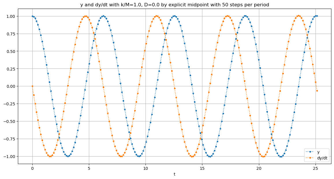
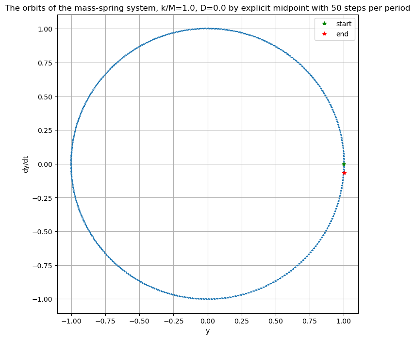
The demos are just for the non-dissipative case, where the solution is known to be \(y = \cos t\), \(dt/dt = -\sin t\).

For a fairer comparison of “accuracy vs computational effort” to the Runge-Kutta method, twice as many time steps are used so that the same number of function evaluations are used for these three methods.

def explicittrapezoid_system(f, a, b, u_0, n):
    """Use the Explict Trapezoid Method (a.k.a Improved Euler)
    to solve system du/dt = f_mass_spring(t, u) for t in [a, b], with initial value u(a) = u_0
    """
    h = (b-a)/n
    t = np.linspace(a, b, n+1)

    # Only the following three lines change for the systems version
    n_unknowns = len(u_0)
    u = np.zeros([n+1, n_unknowns])
    u[0] = np.array(u_0)

    for i in range(n):
        K_1 = f_mass_spring(t[i], u[i])*h
        K_2 = f_mass_spring(t[i]+h, u[i]+K_1)*h
        u[i+1] = u[i] + (K_1 + K_2)/2.
    return (t, u)

M = 1.
k = 1.
D = 0.
u_0 = [1., 0.]
a = 0.
periods = 4
b = 2 * np.pi * periods

stepsperperiod = 50
n = stepsperperiod * periods

(t, U) = explicittrapezoid_system(f_mass_spring, a, b, u_0, n)
y = U[:,0]
Dy = U[:,1]

figure(figsize=[14,7])
title(f"y and dy/dt with {k/M=}, {D=} by explicit trapezoid with {stepsperperiod} steps per period")
plot(t, y, ".:", label="y")
plot(t, Dy, ".:", label="dy/dt")
legend()
xlabel("t")
grid(True)

figure(figsize=[8,8])  # Make axes equal length
title(f"The orbits of the mass-spring system, {k/M=}, {D=} by explicit trapezoid with {stepsperperiod} steps per period")
plot(y, Dy, ":")
xlabel("y")
ylabel("dy/dt")
plot(y[0], Dy[0], "g*", label="start")
plot(y[-1], Dy[-1], "r*", label="end")
legend()
grid(True)

At first glance this is fdoing well, keep the orbits cicular. However note the discrepancy between the start and end points: these should be the same, as they are (visually) the the Runge-Kutta method.

def explicitmidpoint_system(f, a, b, u_0, n):
    """Use the Explicit Midpoint Method (a.k.a Modified Euler)
    to solve system du/dt = f_mass_spring(t, u) for t in [a, b], with initial value u(a) = u_0
    """
    h = (b-a)/n
    t = np.linspace(a, b, n+1)

    # Only the following three lines change for the systems version.
    n_unknowns = len(u_0)
    u = np.zeros([n+1, n_unknowns])
    u[0] = np.array(u_0)

    for i in range(n):
        K_1 = f_mass_spring(t[i], u[i])*h
        K_2 = f_mass_spring(t[i]+h/2, u[i]+K_1/2)*h
        u[i+1] = u[i] + K_2
    return (t, u)

M = 1.
k = 1.
D = 0.
u_0 = [1., 0.]
a = 0.
periods = 4
b = 2 * np.pi * periods

stepsperperiod = 50
n = stepsperperiod * periods

(t, U) = explicitmidpoint_system(f_mass_spring, a, b, u_0, n)
y = U[:,0]
Dy = U[:,1]

figure(figsize=[14,7])
title(f"y and dy/dt with {k/M=}, {D=} by explicit midpoint with {stepsperperiod} steps per period")
plot(t, y, ".:", label="y")
plot(t, Dy, ".:", label="dy/dt")
legend()
xlabel("t")
grid(True)

figure(figsize=[8,8])  # Make axes equal length
title(f"The orbits of the mass-spring system, {k/M=}, {D=} by explicit midpoint with {stepsperperiod} steps per period")
plot(y, Dy, ":")
xlabel("y")
ylabel("dy/dt")
plot(y[0], Dy[0], "g*", label="start")
plot(y[-1], Dy[-1], "r*", label="end")
legend()
grid(True)

---

This work is licensed under Creative Commons Attribution-ShareAlike 4.0 International