

Polynomial Collocation (Interpolation/Extrapolation) and Approximation
Contents
18. Polynomial Collocation (Interpolation/Extrapolation) and Approximation#
Last revised September 24, 2022
References:
Section 3.1 Data and Interpolating Functions of Sauer
Section 3.1 Interpolation and the Lagrange Polynomial of Burden&Faires
Section 4.1 of Chenney&Kincaid
18.1. Introduction#
Numerical methods for dealing with functions require describing them, at least approximately, using a finite list of numbers, and the most basic approach is to approximate by a polynomial. (Other important choices are rational functions and “trigonometric polynomials”: sums of multiples of sines and cosines.) Such polynomials can then be used to aproximate derivatives and integrals.
The simplest idea for approximating \(f(x)\) on domain \([a, b]\) is to start with a finite collection of node values \(x_i \in [a, b]\), \(0 \leq i \leq n\) and then seek a polynomial \(p\) which collocates with \(f\) at those values: \(p(x_i) = f(x_i)\) for \(0 \leq i \leq n\). Actually, we can put the function aside for now, and simply seek a polynomial that passes through a list of points \((x_i, y_i)\); later we will achieve collocation with \(f\) by choosing \(y_i = f(x_i)\).
In fact there are infinitely many such polynomials: given one, add to it any polynomial with zeros at all of the \(n+1\) notes. So to make the problem well-posed, we seek the collocating polynomial of lowest degree.
Theorem Given \(n+1\) distinct values \(x_i\), \(0 \leq i \leq n\), and corresponding \(y\)-values \(y_i\), there is a unique polynomial \(P\) of degree at most \(n\) with \(P(x_i) = y_i\) for \(0 \leq i \leq n\).
(Note: although the degree is typically \(n\), it can be less; as an extreme example, if all \(y_i\) are equal to \(c\), then \(P(x)\) is that constant \(c\).)
Historically there are several methods for finding \(P_n\) and proving its uniqueness, in particular, the divided difference method introduced by Newton and the Lagrange polynomial method. However for our purposes, and for most modern needs, a different method is easiest, and it also introduces a strategy that will be of repeated use later in this course: the Method of Undertermined Coefficients or MUC.
In general, this method starts by assuming that the function wanted is a sum of unknown multiples of a collection of known functions.
Here, \(P(x) = c_0 + c_1 x + \cdots + c_{n-1} x^{n-1} + c_n x^n = \sum_{j=0}^n c_j x^j\).
(Note: any of the \(c_i\) could be zero, including \(c_n\), in which case the degree is less than \(n\).)
The unknown factors (\(c_0 \cdots c_n\)) are the undetermined coefficients.
Next one states the problem as a system of equations for these undetermined coefficients, and solves them.
Here, we have \(n+1\) conditions to be met:
This is a system if \(n+1\) simultaneous linear equations in \(n+1\) unknowns, so the question of existence and uniqueness is exactly the question of whether the corresponding matrix is singular, and so is equivalent to the case of all \(y_i = 0\) having only the solution with all \(c_i = 0\).
Back in terms of polynomials, this is the claim that the only polynomial of degree at most \(n\) with zeros \(x_0 \dots x_n\). And this is true, because any non-trivial polynomial with those \(n+1\) distinct roots is of degree at least \(n+1\), so the only “degree n” polynomial fitting this data is \(P(x) \equiv 0\). The theorem is proven.
The proof of this theorem is completely constructive, and it gives the only numerical method we need.
Briefly, the algorithm is this (indexing from 0 !)
Create the \(n+1 \times n+1\) matrix \(V\) with elements
and the \(n+1\)-element column vector \(y\) with elements \(y_i\) as above.
Solve \(V c = y\) for the vector of coefficients \(c_j\) as above.
I use the name \(V\) because this is called the Vandermonde Matrix.
Enable graph plotting; PyPlot is an interface to the Python package matplotlib.pyplot
If this does not work in a downloaded notebook, see the instructions in the introduction.
using PyPlot
18.2. Example 1#
As usual, I concoct a first example with known correct answer, by using a polynomial as \(f\).
f(x) = 4 + 7x -2x^2 - 5x^3 + 2x^4;
xnodes = [1., 2., 0., 3.3, 4.]  # They do not need to be in order
println("The x nodes 'x_i' are $(xnodes)")
ynodes = f.(xnodes)
println("The y values at the nodes are $(round.(ynodes, sigdigits=6))")  # Rounded for nicer display
The x nodes 'x_i' are [1.0, 2.0, 0.0, 3.3, 4.0]
The y values at the nodes are [6.0, 2.0, 4.0, 62.8192, 192.0]
Julia note 1.
Adding the “point” to the function name (so it is f.(...) instead of f(...)) does vectorization:
the function f is applied “pointwise”, to each element of the input array x_nodes in turn,
with the results returned in an aray of the same size and shape.
See Vectorization of Functions in Notes on the Julia Language.
We will see this again soon.
The Vandermonde matrix:
nnodes = length(xnodes)
n = nnodes-1
V = zeros(nnodes, nnodes)
for i in 0:n
    for j in 0:n
        V[i+1,j+1] = xnodes[i+1]^j  # Shift the array indices up by one, since Julia counts from 1, not 0.
    end
end
Solve, using our functions seen in earlier sections and gathered in Module NumericalMethods
include("NumericalMethods.jl")
using .NumericalMethods: solvelinearsystem, printmatrix
c_A = solvelinearsystem(V, ynodes)
# It helps the visual presentation to round off;
c_A = round.(c_A, sigdigits=6)
println("The coefficients of P are $c_A")
The coefficients of P are [4.0, 7.0, -2.0, -5.0, 2.0]
These are correct!
To compare the computed values P[i] to what they shoudl be (y_nodes[i])
we use the convenient tool zip for looping over two or more “parallel” lists of values:
zip(x,y) effectively produces a list of pairs [(x[1], y[1]), (x[2], y[2]) ...) up till one or both arrays runs out of elements,
and it also works for three or more lists.
We can also check the resulting values of the polynomial:
P = c_A[1] .+ c_A[2]*xnodes + c_A[3]*xnodes.^2 + c_A[4]*xnodes.^3 + c_A[5]*xnodes.^4;
Julia note 2.
The period prefix in the exponential notation .^ and the sum notation `.+ is vectorization and broadcasting:
vectorization of exponentiation: each element of the array is expoentiated in turn, producing an aray of the same size and shape
brodcasting of the addition: that first addition is “number plus array”; the dot indicates that this be done by promoting the number to an array matching the other addend.
Vectorization can also be applied to other binary operations; multiplication in particular.
See the notes on arithmetic operations on arrays in Notes on the Julia Language.
Now we can check the \(y\) values
Julia note 3.
The function zip takes two or more arrays (preferably of the same size and shape) and turns them into an array with each element a tuple of values, one from the corresponding position in each input array.
For example, with 1D arrays x and y of length n, zip(x, y) is [ ( x[1], y[1] ), ( x[2], y[2] ) ... ( x[n], y[n] ) ]
for (x, y, P_i) in zip(xnodes, ynodes, P)
    println("P($x) should be $(round(y, sigdigits=6)); it is $(round(P_i, sigdigits=6))")
end
P(1.0) should be 6.0; it is 6.0
P(2.0) should be 2.0; it is 2.0
P(0.0) should be 4.0; it is 4.0
P(3.3) should be 62.8192; it is 62.8192
P(4.0) should be 192.0; it is 192.0
18.3. Functions for computing the coefficients and evaluating the polynomials#
We will use this procedure several times, so it time to put it into a functions.
The names polyfit and polyval come from very similar functions that are standard in Python and Matlab.
We also add a pretty printer for polynomials, and import the pretty printer printmatrix for matrices.
function polyfit(x, y)
    # Compute the coeffients c_i of the polynomial of lowest degree that collocates the points (x[i], y[i]).
    # These are returned in an array c of the same length as x and y, even if the degree is less than the normal length(x)-1,
    # in which case the array has some trailing zeroes.
    # The polynomial is thus p(x) = c[1] + c[2]x + ... c[n+1] x^n where n=length(x)-1, the nominal degree.

    nnodes = length(x)
    n = nnodes - 1
    V = zeros(nnodes, nnodes)
    for i in 0:n
        for j in 0:n
             V[i+1,j+1] = x[i+1]^j  # Shift the array indices up by one, since Julia counts from 1, not 0.
        end
    end
    c = solvelinearsystem(V, y)
    return c
end;
function polyval(x; coeffs)  # coeffs has to be a keyword argument in order that only x gets vectorized
    # Evaluate the polynomial with coefficients in c (as given by polyfit, for example).
    n = length(coeffs) - 1
    powers = collect(0:n)  # function collect turns the "AbstractRange" 0:n into an array of numbers.
    y = sum(coeffs .* x.^powers)
    return y
end;
function displaypolynomial(c; sigdigits=6)
    # Note that the function "print" does not end by going to a new line as `println` does;
    # this is useful when you want to create a line of output piece-by-piece, as done here.

    c = round.(c, sigdigits=sigdigits) # Clean up by rounding to sigdigits significant digits; yes, that's vectorization again.
    degree=length(c)-1
    print("P_$(degree)(x) = ")
    print(c[1])
    if degree > 0
        c_1 = c[2]
        if c_1 > 0
            print(" + $(c_1)x")
        elseif coeff < 0
            print(" - $(-c_1) x")
        end
    end
    if degree > 1
        for j in 2:degree
            c_j = c[j+1]
            if c_j > 0
                print(" + $(c_j)x^$j")
            elseif c_j < 0
                print(" - $(-c_j)x^$j")
            end
            # Note: if c_j=0, there is nothing to say.
         end
    end
    println()
end;
18.4. Example B: \(f(x)\) not a polynomial of degree \(\leq n\)#
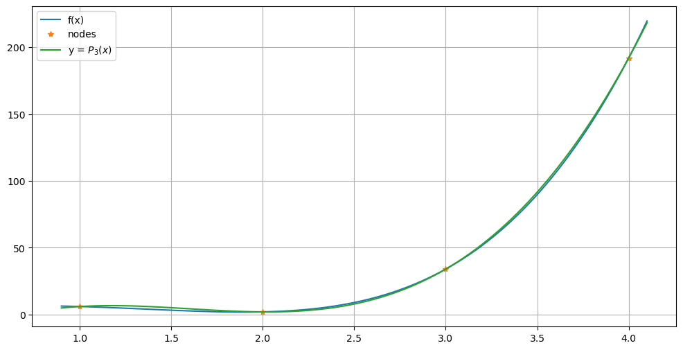
Reduce the degree of the interpolating \(P\) to three by using only four nodes:
xnodes = [1., 2., 3., 4.];
println("The x nodes 'x_i' are $xnodes")
ynodes = f.(xnodes)
println("The y values at the nodes are $ynodes")
c_B = polyfit(xnodes, ynodes);
displaypolynomial(c_B)
The x nodes 'x_i' are [1.0, 2.0, 3.0, 4.0]
The y values at the nodes are [6.0, 2.0, 34.0, 192.0]
P_3(x) = -44.0 + 107.0x - 72.0x^2 + 15.0x^3
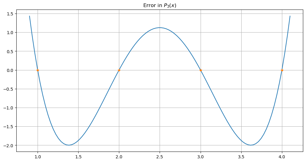
There are several ways to assess the accuracy of this fit; we start graphically, and later consider the maximum and root-mean-square (RMS) errors.
xplot = range(0.9, 4.1, 100)  # for graphing: go a bit beyond the nodes
fplot = f.(xplot);
Pplot = polyval.(xplot, coeffs=c_B);
figure(figsize=[12,6])
plot(xplot, fplot, label="f(x)")
plot(xnodes, ynodes, "*", label="nodes")
plot(xplot, Pplot, label=L"y = $P_3(x)$")
legend()
grid(true);
Perror = fplot - Pplot
figure(figsize=[12,6])
title(L"Error in $P_3(x)$")
plot(xplot, Perror)
plot(xnodes, zero(xnodes), "*")
grid(true)
18.5. Example C: \(f(x)\) not a polynomial at all#
g(x) = exp(x)
a_g = -1.0
b_g = 1.0;
degree = 4
n_nodes = degree + 1

xnodes = range(a_g, b_g, n_nodes)
gnodes = g.(xnodes)
c_C = polyfit(xnodes, gnodes)
println("node x values $xnodes")
println("node y values $(round.(gnodes, sigdigits=4))")
displaypolynomial(c_C, sigdigits=4)
node x values -1.0:0.5:1.0
node y values [0.3679, 0.6065, 1.0, 1.649, 2.718]
P_4(x) = 1.0 + 0.9979x + 0.4996x^2 + 0.1773x^3 + 0.04344x^4
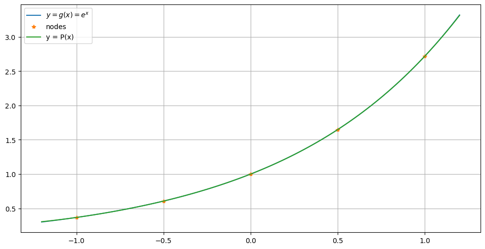
For comparison, the degree 4 Taylor polynomial for \(e^x\) with center 0 is (to the same 6 significant digits)
xplot = range(a_g - 0.2, b_g + 0.2, 100)  # Go a bit beyond the nodes in each direction
gplot = g.(xplot)
Pplot_g = polyval.(xplot, coeffs=c_C);
figure(figsize=[12,6])
plot(xplot, gplot, label=L"y = g(x) = e^x")
plot(xnodes, gnodes, "*", label="nodes")
plot(xplot, Pplot_g, label="y = P(x)")
legend()
grid(true)
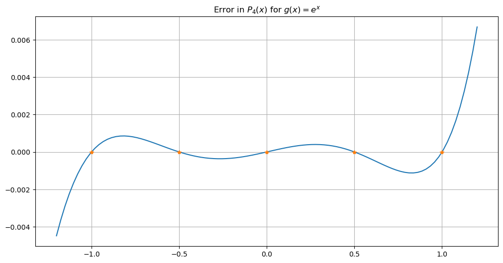
Perror_g = gplot - Pplot_g
figure(figsize=[12,6])
degree = 8
title(L"Error in $P_4(x)$ for $g(x) = e^x$")
plot(xplot, Perror_g)
plot(xnodes, zero(xnodes), "*")
grid(true)
This work is licensed under Creative Commons Attribution-ShareAlike 4.0 International